ChromaDB vs Milvus: Vector Databases for Scale
At 50 million vector embeddings, the architectural shortcut you picked during a weekend hackathon turns into a production outage. Selecting a vector database isn't about running basic cosine similarity queries on local data—it's a high-stakes decision about memory allocation, query throughput, horizontal scale, and index re-building under heavy write loads.
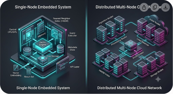
ChromaDB and Milvus sit at opposite ends of the vector database design spectrum. ChromaDB prioritizes developer ergonomics, zero-config local prototyping, and rapid embedded workflows. Milvus was engineered from day one as a cloud-native, distributed, multi-node engine built to handle billions of high-dimensional vectors with strict sub-50-millisecond SLA requirements.
Here is the bottom-line verdict: If you are building an early-stage prototype, a single-tenant agent, or managing under 10 million embeddings on a single server, ChromaDB offers the fastest path to production. If you are serving multi-tenant enterprise RAG applications, ingesting millions of dynamic vectors daily, or scaling past 50 million embeddings, Milvus is the mandatory architectural choice despite its higher operational overhead.
In this deep dive, we will break down the underlying architecture, indexing algorithms, memory footprints, and practical resource costs of both platforms so you can make the right infrastructure call the first time.
Core Architectural Differences: Embedded Simplicity vs. Cloud-Native Clusters
Understanding how ChromaDB and Milvus process, index, and query vector data requires looking under the hood of their architectural paradigms.
ChromaDB Architecture: SQLite, DuckDB, and Local State
ChromaDB started as an embedded, developer-first vector store written in Python and C++. In its single-node mode, it runs directly inside your application process or as a lightweight standalone Docker container.
ChromaDB relies on standard local persistence engines:
- Metadata and System State: Managed via SQLite.
- Vector Storage and Indexing: Built on top of hnswlib, a lightweight C++ implementation of Hierarchical Navigable Small World (HNSW) graphs.
- Query Engine: Executes in-process, reading vectors from disk or cached RAM blocks.
While ChromaDB has introduced distributed and hosted options, its native strength remains simple deployment. You install it with pip install chromadb, point it to a local directory, and immediately start appending embeddings. The trade-off is structural: because metadata operations bottleneck through SQLite and vector index modifications happen in-memory on a single node, scaling past tens of millions of vectors requires scaling up hardware (RAM and CPU) rather than adding nodes.
Milvus Architecture: Disaggregated Storage and Compute
Milvus operates on a cloud-native, microservices-based architecture designed to decouple storage from compute completely. Instead of running as a monolith, a Milvus cluster breaks down into stateless specialized components:
- Access Layer: Handles client connections, query parsing, and rate limiting.
- Coordinator Service: Manages cluster topology, task allocation, and metadata state using etcd.
- Worker Nodes: Divided into Query Nodes (handling search execution), Data Nodes (handling batch ingestion), and Index Nodes (building complex graph/IVF indexes asynchronously).
- Object Storage: Relies on AWS S3, Google Cloud Storage, or MinIO for long-term persistence, keeping raw vector data isolated from computational compute nodes.
When you insert vectors into Milvus, they land in an append-only log backed by Apache Pulsar or Kafka. Data is streamed, persisted to object storage in segments, and indexed asynchronously. This decoupling ensures that a massive burst of incoming writes will never degrade ongoing search queries on Query Nodes.
Indexing Algorithms and Search Performance
Vector databases rely on Approximate Nearest Neighbor (ANN) search algorithms to query high-dimensional space without performing expensive brute-force brute-scan operations across every single vector.
| Index Approach | Primary Algorithm Types | Memory Footprint | Key Performance Trade-off |
|---|---|---|---|
| In-Memory Graph | HNSW (Default in ChromaDB) | High RAM Usage | Delivers ~98%+ recall with sub-10ms latency; requires keeping full graph in memory. |
| Inverted File / Quantized | IVF_FLAT, IVF_PQ (Native in Milvus) | Compressed RAM Usage | Reduces memory consumption up to 80%; trades minor recall accuracy for higher throughput. |
ChromaDB Indexing Mechanics
ChromaDB uses HNSW as its core indexing mechanism. HNSW creates a multi-layered graph where the top layers feature long-range connections for fast routing, and the bottom layers feature dense, short-range connections for precise neighbor identification.
- Recall Accuracy: Exceptionally high (typically 95% to 99% recall depending on parameters like M and efConstruction).
- Latency: Sub-10ms response times for small to medium datasets.
- The Bottleneck: HNSW graphs must reside entirely in RAM during search queries. Furthermore, updating an HNSW graph dynamically when inserting new vectors causes lock contention and memory fragmentation. In ChromaDB, rebuilding or expanding this graph on a single server under continuous heavy writes leads to sharp latency spikes.
Milvus Indexing Diversity

Milvus supports a wide variety of index types, allowing system architects to tune memory usage, write throughput, and search latency:
- HNSW: Ideal for high-recall requirements where ample RAM is available.
- IVF_FLAT (Inverted File Flat): Groups vectors into Voronoi cells using k-means clustering. It narrows down search spaces rapidly, consuming less memory than pure HNSW graphs.
- IVF_PQ (Product Quantization): Compresses high-dimensional floating-point vectors into compact byte codes. This reduces memory usage by up to 75-80% at the cost of a slight drop in search recall accuracy.
- DiskANN: An advanced disk-based indexing algorithm developed to run billion-scale vector searches directly from fast NVMe SSDs, keeping RAM requirements surprisingly low.
Milvus processes index construction out-of-band using dedicated Index Nodes. This prevents heavy background re-indexing tasks from slowing down live application queries.
Side-by-Side Architectural Matrix
To see how both platforms stack up across core technical capabilities, refer to the comparison table below:
| Capability / Metric | ChromaDB | Milvus |
|---|---|---|
| Primary Architecture | Embedded / Single-Node Monolith | Cloud-Native / Disaggregated Microservices |
| Storage Backend | SQLite + Local Disk | MinIO / AWS S3 / Azure Blob + etcd |
| Message / Event Queue | None (Direct In-Memory / File Writes) | Apache Pulsar / Kafka |
| Supported Indexes | HNSW (via hnswlib) | HNSW, IVF_FLAT, IVF_PQ, DiskANN, SCaNN, GPU Indexes |
| Scaling Strategy | Scale Up (Vertical CPU/RAM) | Scale Out (Horizontal Node Auto-scaling) |
| Filtering Capabilities | Basic Metadata Filtering (SQL-like) | Advanced Dynamic Schema & Boolean Expressions |
| Multi-Tenancy | Partitioning via Separate Collections | Partition Keys, Multi-Database, Collection Segregation |
| Operational Overhead | Minimal (Zero-config setup) | High (Requires Kubernetes / Helm / Storage Management) |
| Optimal Vector Range | < 10 Million Vectors | 10 Million to 1 Billion+ Vectors |
| GPU Acceleration | Limited / Non-standard | Native CUDA Support for Indexing & Queries |
Data Ingestion, Write Scalability, and Index Building
In real-world RAG applications, vector databases do not operate in a read-only environment. Enterprise pipelines continuously chunk documents, embed new text, update existing metadata, and drop outdated documents.
Real-time Write Contention in ChromaDB
When pushing large streaming batches into ChromaDB, the system performs two actions simultaneously: appending record metadata to SQLite and updating the HNSW graph files.
At modest scale (e.g., inserting 1,000 vectors per minute), ChromaDB handles this effortlessly. However, as dataset size passes 5 million vectors, concurrent read and write operations create an architectural bottleneck:
- Locking: SQLite write locks delay incoming metadata writes.
- Graph Re-building: In-memory graph mutations force CPU cores to execute graph re-balancing routines, causing search queries running on the same process to queue up.
Stream Ingestion in Milvus
Milvus handles writes using a streaming log architecture. When you insert a batch of 100,000 vectors into Milvus:
- The request lands instantly on the Proxy Layer, which validates schema and writes the batch to Pulsar or Kafka.
- Data Nodes pull the log stream and write un-indexed vector batches into immutable memory segments (Growing Segments).
- Once a segment reaches its size threshold (typically 512MB), it is sealed and written to cloud object storage as a Sealed Segment.
- Index Nodes asynchronously pull sealed segments, build the requested index (e.g., HNSW or IVF_PQ), and write the finalized index files back to object storage.
- Query Nodes load the newly built index into RAM for query execution.
Because ingestion is completely decoupled from indexing and querying, search performance stays consistent even when processing millions of writes per hour.
Deploying to Production: Resource Management and Operational Realities
Choosing a vector database requires balancing operational complexity against technical capabilities. A system that is easy to deploy locally might become difficult to manage at scale, while a system built for enterprise scale brings initial operational overhead.
| Deployment Parameter | ChromaDB Production Path | Milvus Distributed Path |
|---|---|---|
| Infrastructure Complexity | Low (Runs in App Container or Docker) | High (Requires Kubernetes Cluster & Helm) |
| Scale Bounds | Single-Node Hardware Limits | Horizontal Auto-scaling across Worker Nodes |
| Setup Duration | Instant single-command startup | Multi-service enterprise cluster setup |
Running ChromaDB in Production
Deploying ChromaDB is straightforward. You can run it directly as an embedded module within a FastAPI service or deploy its official Docker container to AWS ECS, GCP Cloud Run, or a standard Virtual Machine.
python import chromadb from chromadb.config import Settings
Connect to persistent Chroma instance
client = chromadb.HttpClient(host="localhost", port=8000)
Create or retrieve collection with cosine similarity
collection = client.get_or_create_collection( name="enterprise_knowledge_base", metadata={"hnsw:space": "cosine"} )
Upsert vectors with metadata
collection.upsert( ids=["doc_102", "doc_103"], embeddings=[[0.12, -0.43, 0.88], [0.05, 0.11, -0.29]], metadatas=[{"department": "finance", "year": 2026}, {"department": "hr", "year": 2025}], documents=["Q3 Financial Report...", "Employee Handbook..."] )
Resource Considerations for ChromaDB:
- Memory Overhead: You must allocate enough RAM to keep the HNSW index of every active collection in memory. For 10 million vectors of 1,536 dimensions (OpenAI text-embedding-3-large format), raw uncompressed vector storage requires roughly 60 GB of RAM, plus an additional 20-30% buffer for HNSW graph structures.
- CPU Allocation: Single-thread operations handle small queries quickly, but multi-tenant query surges require provisioning large multi-core instances (e.g., AWS c6i.8xlarge).
Running Milvus in Production
Milvus deployment requires container orchestration infrastructure. While Milvus offers a standalone Docker image for local development, production environments require deploying Milvus Distributed via Kubernetes using Helm charts or the Milvus Operator.

python from pymilvus import connections, Collection, FieldSchema, CollectionSchema, DataType
Connect to Milvus Cluster Proxy
connections.connect("default", host="milvus-proxy.internal.net", port="19530")
Define Schema explicitly for high-throughput scaling
fields = [ FieldSchema(name="id", dtype=DataType.VARCHAR, is_primary=True, max_length=64), FieldSchema(name="tenant_id", dtype=DataType.VARCHAR, max_length=32), FieldSchema(name="embedding", dtype=DataType.FLOAT_VECTOR, dim=1536) ]
schema = CollectionSchema(fields, description="Multi-tenant Enterprise Vectors") collection = Collection("enterprise_rag", schema)
Create IVF_PQ Index for optimized memory footprint
index_params = { "metric_type": "COSINE", "index_type": "IVF_PQ", "params": {"nlist": 2048, "m": 16, "nbits": 8} } collection.create_index(field_name="embedding", index_params=index_params)
Infrastructure Dependencies for Milvus Distributed:
- Kubernetes Cluster: Minimum 3 worker nodes recommended for high availability.
- etcd Cluster: Manages state metadata and node registration across the cluster.
- MinIO / Cloud Object Storage: Persists immutable vector log segments.
- Apache Pulsar / Kafka: Serves as the high-throughput message backbone.
Maintaining this ecosystem requires Kubernetes administration experience. If your engineering team lacks dedicated DevOps resources, running self-hosted Milvus cluster instances introduces operational complexity.
Common Architectural Pitfalls and How to Avoid Them
Pitfall 1: Neglecting Memory Footprint Calculations
Engineers often calculate memory needs by multiplying vector count by dimensionality size (50,000,000×1,536×4 bytes?307 GB). They then provision a 320 GB RAM server, assuming it will comfortably handle the load.
The Reality: Graph-based indexes like HNSW add significant overhead for node links and routing vectors—often requiring 1.2x to 1.5x the raw vector size. Additionally, operating system processes, metadata caching, and execution buffers need dedicated headroom. Running out of memory causes the OS OOM killer to terminate your database process.
Solution: If using ChromaDB, provision at least 2x the raw vector size in system RAM. If using Milvus, leverage memory compression techniques like IVF_PQ or offload cold vectors to disk using DiskANN to keep infrastructure costs manageable.
Pitfall 2: Over-Filtering Metadata on Low-Cardinality Fields
Applying restrictive metadata filters (e.g., WHERE tenant_id = 'user_9921') alongside vector similarity searches can cause unexpected performance slowdowns if configured incorrectly.
The Reality: If your database runs vector similarity first and filters metadata second, it may scan the top 100 nearest neighbors, discover only 2 match the metadata filter, and return an incomplete result set. Conversely, if it runs metadata filtering first without proper indexes, it falls back to a full table scan.
Solution: Milvus supports native scalar indexing and bitset filtering, executing boolean pre-filtering before running vector distance algorithms. In ChromaDB, keep metadata payloads small and avoid deep nested JSON filtering structures across high-cardinality fields.
Practical Benchmarks: When to Scale Up vs. Scale Out
To determine the practical limits for each database, consider these performance thresholds based on vector volume and concurrency requirements.
Scale Tier 1: 100,000 to 5 Million Vectors
- Target Use Cases: Internal documentation search, customer support chatbots, small-scale semantic search engines.
- Recommended Tool: ChromaDB
- Why: ChromaDB handles this volume on a modest virtual machine (4 vCPUs, 16GB RAM) with single-digit millisecond query latencies. Setting up a distributed Milvus cluster for this volume introduces unnecessary infrastructure complexity.
Scale Tier 2: 5 Million to 50 Million Vectors
- Target Use Cases: Multi-tenant SaaS products, enterprise knowledge graphs, automated code indexing tools.
- Recommended Tool: ChromaDB (Scaled Up) or Milvus (Standalone/Managed)
- Why: At this stage, single-node ChromaDB requires high-spec hardware (64GB+ RAM, fast NVMe drives) and carefully managed read/write workloads. If your team prefers low operational maintenance, running ChromaDB on a high-spec instance works well. However, if you require non-blocking ingestion alongside live queries, transitioning to Milvus becomes advantageous.
Scale Tier 3: 50 Million to 1 Billion+ Vectors
- Target Use Cases: E-commerce recommendation engines, global threat detection systems, large-scale multimodal retrieval systems.
- Recommended Tool: Milvus (Distributed Cluster)
- Why: ChromaDB's single-node model encounters hardware limits at this scale. Milvus distributes vectors across dozens of Query Nodes, streams inserts through Pulsar, and persists data to object storage, allowing you to scale read and write capacity independently.
Final Decision Matrix: Which Vector Database Should You Pick?
To guide your technical decision, select the scenario below that best matches your project requirements:
Choose ChromaDB if:
- You are building a prototype, MVP, or internal tool that needs to launch quickly.
- Your vector collection is expected to stay below 10 million embeddings.
- You want an embedded vector store that runs locally inside Python, TypeScript, or desktop environments.
- Your team lacks dedicated DevOps or Kubernetes management resources.
- You prefer a simple, single-command setup without managing external services like etcd or object storage.
Choose Milvus if:
- You are architecting an enterprise system scaling beyond 50 million embeddings.
- You need to support concurrent read/write workloads without performance degradation.
- You require granular control over indexing algorithms (IVF_FLAT, IVF_PQ, DiskANN, GPU acceleration) to optimize RAM costs.
- You are building a multi-tenant application requiring robust metadata filtering and dynamic partitioning.
- Your team runs infrastructure on Kubernetes and can manage distributed cloud architectures.
Selecting the right vector database comes down to matching its architecture to your project's operational realities. Starting simple with ChromaDB lets you build quickly; transitioning to Milvus gives you the horizontal scale required for high-volume production systems.
For hands-on evaluation guides and architectural comparisons of modern developer platforms, explore the rest of our technical reviews on Saasbonus.