LanceDB vs ChromaDB: Best Embedded Vector DB for AI
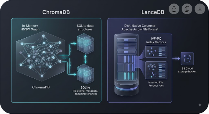
Choosing between LanceDB and ChromaDB comes down to a single engineering decision: do you need an in-memory vector store for rapid prototyping, or a disk-native columnar engine that scales without crashing your server when RAM runs out?
As Generative AI systems transition from local prototypes to production pipelines, the vector database quickly becomes an infrastructure bottleneck. Embedded vector databases run directly inside your application process or access local storage, removing the network latency, API costs, and cluster management that come with cloud-managed vector stores like Pinecone or Milvus.
Two engines lead the open-source embedded landscape: ChromaDB and LanceDB. Both let you store and query high-dimensional embeddings using Python or JavaScript APIs. Their underlying storage layouts, indexing strategies, and memory profiles are completely different.
At Saasbonus, we tested both engines across synthetic benchmarks and production-style retrieval-augmented generation (RAG) workloads. This guide breaks down their core architectures, memory footprints, query capabilities, and operational trade-offs so you can select the right vector engine for your stack.
Core Architecture: How LanceDB and ChromaDB Store Vectors
To understand why these engines diverge under heavy load, you have to look at how each system writes and queries vectors on disk and in memory.
How ChromaDB Works Under the Hood
ChromaDB focuses on developer velocity and rapid setup. It uses a decoupled architecture that splits metadata persistence from vector indexing:
- Metadata and Collection Storage: ChromaDB relies on SQLite to handle document collections, metadata key-value pairs, and structural configurations. SQLite gives ChromaDB simple file persistence and transactional safety.
- Vector Indexing: For approximate nearest neighbor (ANN) search, ChromaDB uses HNSWlib, a C++ implementation of the Hierarchical Navigable Small World (HNSW) graph algorithm. HNSW builds multi-layer graph networks where nodes represent vectors and edges represent spatial proximity.
- Query Execution: Similarity searches navigate the HNSW graph to find nearest neighbors. Because graph traversal requires fast random memory lookups, the entire active HNSW index structure must reside directly in RAM.
This setup lets developers install and run ChromaDB in seconds. The trade-off is direct coupling between dataset size and RAM usage.
How LanceDB Works Under the Hood
LanceDB builds directly on the Lance file format, an open-source columnar data layout created specifically for machine learning workflows and multimodal datasets. Lance serves as a modern alternative to Parquet, optimized for random disk access and high-dimensional vector search.
- Apache Arrow Core: Lance integrates natively with Apache Arrow. Data resides in a columnar format that enables zero-copy data sharing across Python, Rust, JavaScript, and analytical query engines like DuckDB or Polars.
- Disk-Native Indexing: Rather than loading complete graphs into memory, LanceDB uses Inverted File with Product Quantization (IVF-PQ) and disk-based index structures. Product quantization compresses high-dimensional vectors into compact byte codes. LanceDB then evaluates distance calculations directly against disk-mapped memory (NVMe SSDs or object stores like Amazon S3).
- Unified Dataset File: Metadata, raw text payloads, binary files (images, audio, video), and vector embeddings sit inside the same unified Lance dataset file. It does not require an external relational store like SQLite.
By decoupling search speed from active memory footprint, LanceDB queries millions of records using a tiny memory footprint.
Performance and Memory Footprint: Navigating the Memory Wall
Evaluating vector databases usually starts with query latency, measured in milliseconds per lookup. In production environments, RAM consumption and ingestion throughput drive operational stability and infrastructure costs.
RAM Footprint: In-Memory HNSW vs Disk-Native IVF-PQ
Consider a production workload containing 5 million document chunks embedded with OpenAI's `text-embedding-3-large` model (1,536 float32 dimensions).
- Uncompressed Math: 5,000,000 vectors 1,536 dimensions 4 bytes per float32 = 30.72 GB of raw vector data.
- ChromaDB Overhead: Holding an active HNSW graph for 5 million vectors in memory requires storing both raw floating-point values and graph pointers. Total system RAM usage typically climbs to between 45 GB and 60 GB. If the host machine runs out of memory, the process crashes or suffers heavy swapping penalties.
- LanceDB Overhead: Through IVF-PQ quantization, LanceDB compresses 1,536-dimensional vectors into compact sub-vectors. The active index footprint drops down to 1.5 GB to 3 GB of memory. Uncompressed vector data stays on NVMe storage, accessed via memory-mapped I/O when needed.
For datasets under 500,000 vectors, ChromaDB delivers sub-5 millisecond response times because every vector sits pre-loaded in system memory. Once datasets pass millions of records, LanceDB avoids out-of-memory errors while keeping latencies under 15 milliseconds.
Ingestion Throughput and Index Building
Ingestion speed involves two operations: writing raw records to storage and building the search index.
- ChromaDB Ingestion: Small batches write quickly. As the HNSW graph grows, inserting new records requires calculating vector distances against existing graph nodes to establish edges. Indexing time grows non-linearly as total volume increases.
- LanceDB Ingestion: LanceDB writes raw Arrow record batches directly to disk at hundreds of thousands of rows per second. IVF-PQ index creation can be delayed until batch writes complete. Parallel Rust execution and SIMD instructions allow fast index creation on multi-core hardware.
Feature Comparison: LanceDB vs ChromaDB
The table below contrasts key architectural features between ChromaDB and LanceDB:
| Feature | ChromaDB | LanceDB |
|---|---|---|
| Primary Architecture | Embedded / Client-Server | Embedded / Serverless / Lakehouse |
| Storage Engine | SQLite + HNSWlib | Apache Arrow + Lance Columnar Format |
| Default Index Types | In-Memory HNSW, SPANN | IVF-PQ, IVF-HNSW-PQ, BTree |
| Storage Target | System RAM + Local SQLite File | Local NVMe / SSD, Amazon S3, Azure Blob, GCS |
| Memory Usage | High (RAM holds full HNSW graph) | Low (Disk-native, memory-mapped vectors) |
| Multimodal Support | Metadata references / URL pointers | Native storage for images, audio, video, and text |
| Data Versioning | No native dataset versioning | Built-in zero-copy versioning and time travel |
| Metadata Filtering | Python dictionary filters | SQL pushdown via DataFusion and DuckDB |
| Ecosystem Hooks | LangChain, LlamaIndex, Haystack | DuckDB, Polars, PyTorch, Ray, Spark, LangChain |
| Supported Languages | Python, JavaScript/TypeScript | Python, JavaScript/TypeScript, Rust, Go |
| Open Source License | Apache 2.0 | Apache 2.0 |
Metadata Filtering and Query Capabilities
Production RAG systems rarely perform unconstrained vector searches. Applications need to isolate vectors by tenant ID, user permissions, creation dates, or content tags.

How a database processes metadata filters determines whether search requests finish in milliseconds or seconds.
Filtering Vectors in ChromaDB
ChromaDB provides a dictionary-based query syntax for metadata filtering, using standard comparison operators like `$eq`, `$gt`, `$in`, `$and`, or `$or`:
```python
ChromaDB Filtering Example
results = collection.query( query_embeddings=[[0.12, -0.43, 0.89]], n_results=5, where={"category": "financial_report"}, where_document={"$contains": "Q3 2026"} ) ```
ChromaDB evaluates filter expressions against SQLite or applies post-filtering to returned similarity scores. On highly restrictive filters (such as matching less than 1% of total records), post-filtering can cause recall drops if candidate vectors are discarded after graph traversal finishes.
SQL Filtering and Pushdown in LanceDB
Because LanceDB stores metadata fields in the same columnar Arrow structure as vector embeddings, it processes filters using DataFusion, an open-source Rust SQL engine:
```python
LanceDB Filtering Example
results = ( table.search([0.12, -0.43, 0.89]) .where("category = 'financial_report' AND created_at >= '2026-01-01'", prefilter=True) .limit(5) .to_pandas() ) ```
Setting `prefilter=True` forces LanceDB to execute filter pushdown at the storage layer before distance calculations occur. This preserves search recall across narrow metadata queries while scanning only matching disk segments.
Through native DuckDB integration, developers can also query Lance datasets using standard SQL:
```sql -- Executing SQL search over a LanceDB dataset inside DuckDB SELECT id, text, vector_distance(vector, [0.12, -0.43, 0.89]) AS distance FROM lance_vector_search('s3://my-bucket/rag_data.lance', 'vector', [0.12, -0.43, 0.89]) WHERE tenant_id = 'tenant_8841' ORDER BY distance ASC LIMIT 5; ```
This integration lets engineering teams run analytics, join tables, and aggregate fields directly over vector storage.
Multimodal Data Support and Arrow Integration
AI retrieval pipelines increasingly handle multimodal data, including text, source code, document scans, audio clips, and image frames.
The Multimodal Bottleneck in SQLite Stores
In systems like ChromaDB, storing large binary assets (such as a 3 MB image or PDF render) inside SQLite degrades database performance. Teams usually store assets in S3 buckets, log URL references inside ChromaDB metadata, and handle file fetching manually in application code.
LanceDB's Native Multimodal Handling
LanceDB stores binary media natively inside its columnar layout:
- Unified Schema: A single table schema can store text strings, float32 vector embeddings, and raw image bytes alongside one another.
- Lazy Binary Reading: LanceDB uses lazy evaluations. When searching vector spaces across thousands of image embeddings, it reads only vector columns during search and fetches binary payload bytes for the final top matched records.
- Zero-Copy Conversion: Arrow memory layouts let retrieved vector data pass directly into PyTorch tensors, Polars DataFrames, or Ray datasets without serialization overhead.
For computer vision and document processing systems, this layout removes the need to maintain separate object stores and feature databases.
SDK Integration and Ecosystem Support
Both projects feature clean developer APIs while serving different operational needs.
ChromaDB: Fast Setup for Early Prototypes
ChromaDB works well for simple setups and early experimentation:
- Simple Installation: A single `pip install chromadb` command sets up the database.
- Framework Defaults: ChromaDB serves as a default option in tutorials for LangChain, LlamaIndex, and AutoGen. Built-in helpers automatically convert raw strings to embeddings using OpenAI, Hugging Face, or local model endpoints.
LanceDB: Scalable Infrastructure for Production
LanceDB provides structured control over disk indices, schemas, and cloud deployment:
- Serverless Deployments: A LanceDB store consists of `.lance` files on local storage or object stores. Applications can run LanceDB inside AWS Lambda functions, container instances, or edge devices while querying S3 data directly.
- Built-in Dataset Versioning: Writes, updates, and deletes in LanceDB produce immutable version states. Teams can query historical snapshot states, audit changes, or revert updates without setting up custom backup pipelines.
- Language SDKs: LanceDB maintains native libraries for Python, JavaScript/Node.js, Rust, and Go.
Hands-On Code: Setup and Vector Searching
The examples below show how to initialize storage, write document embeddings, and execute filtered similarity queries in Python.
Running Vector Search with ChromaDB
```python import chromadb from chromadb.utils import embedding_functions
1. Initialize local persistent client
client = chromadb.PersistentClient(path="./chroma_db_data")
2. Configure embedding function

openai_ef = embedding_functions.OpenAIEmbeddingFunction( api_key="your-api-key", model_name="text-embedding-3-small" )
3. Create or fetch document collection
collection = client.get_or_create_collection( name="knowledge_base", embedding_function=openai_ef )
4. Insert documents and metadata
collection.add( documents=[ "LanceDB uses columnar storage for fast vector lookups.", "ChromaDB relies on SQLite and HNSW for local search." ], metadatas=[ {"category": "database", "author": "dev_team"}, {"category": "database", "author": "research_team"} ], ids=["doc_1", "doc_2"] )
5. Search vectors with metadata filter
results = collection.query( query_texts=["How does columnar storage work?"], n_results=1, where={"category": "database"} )
print(results["documents"]) ```
Running Vector Search with LanceDB
```python import lancedb from lancedb.pydantic import LanceModel, Vector from lancedb.embeddings import get_registry
1. Select embedding model from registry
func = get_registry().get("openai").create(name="text-embedding-3-small")
2. Define schema with Pydantic
class DocumentSchema(LanceModel): id: str text: str = func.SourceField() vector: Vector(func.ndims()) = func.VectorField() category: str author: str
3. Connect to database path (or s3://bucket/path)
db = lancedb.connect("./lancedb_data")
4. Create table using schema
table = db.create_table("knowledge_base", schema=DocumentSchema, mode="overwrite")
5. Insert records (embeddings generate automatically)
data = [ { "id": "doc_1", "text": "LanceDB uses columnar storage for fast vector lookups.", "category": "database", "author": "dev_team" }, { "id": "doc_2", "text": "ChromaDB relies on SQLite and HNSW for local search.", "category": "database", "author": "research_team" } ] table.add(data)
6. Build disk index for large-scale retrieval (IVF-PQ)
table.create_index(num_partitions=2, num_sub_vectors=1)
7. Execute query with SQL pre-filtering
results = ( table.search("How does columnar storage work?") .where("category = 'database'", prefilter=True) .limit(1) .to_pandas() )
print(results[["id", "text", "category"]]) ```
Both APIs are clean and straightforward. LanceDB adds explicit control over schema configurations, index timing, and SQL filter execution.
When to Choose ChromaDB
ChromaDB is a great fit for specific development stages and light workloads:
- Early Prototypes and Demos: Building proof-of-concept projects or hackathon apps that need minimal setup time.
- Small Text Datasets: Applications managing under 500,000 vectors (less than 5 GB total storage) that fit easily into system RAM.
- Quick Framework Setup: Projects using LangChain or LlamaIndex defaults where setting up disk storage parameters isn't necessary.
- Basic Metadata Tagging: Workloads that only need simple key-value filtering without analytical SQL support.
When to Choose LanceDB
LanceDB provides the performance needed for production systems and scaling vector infrastructure:
- Large Vector Datasets (Millions of Records): Applications that exceed available system memory and require disk-native indexing to lower hardware costs.
- Multimodal Content Processing: Storing text, image, audio, or PDF data directly alongside vector embeddings in unified tables.
- Serverless and Cloud Architecture: Running vector search inside edge functions, AWS Lambda, or container services reading directly from cloud object stores.
- Data Lakehouse Workflows: Joining vector search outputs with relational datasets through DuckDB, Polars, or Apache Arrow integrations.
- Data Auditing and Versioning: Workflows requiring snapshot history, zero-copy versions, and rollback support.
How to Migrate from ChromaDB to LanceDB
As RAG applications grow, teams often start with ChromaDB for initial prototypes and shift to LanceDB when hit by high memory usage in production.
Here is a 4-step process for migrating vector data safely:
- Export Collections: Extract documents, embeddings, and metadata out of ChromaDB collections into Pandas DataFrames or Arrow record batches using Chroma's SDK.
- Define Lance Schemas: Build explicit Pydantic or Arrow schemas in LanceDB mapping `id`, `document`, `metadata`, and `embedding` fields into typed columns.
- Batch Ingestion: Stream records into LanceDB in batches of 50,000 to 100,000 using zero-copy Arrow writes rather than single-record appends.
- Build Disk Indexes: Once ingestion finishes, trigger index generation (`table.create_index()`) specifying `IVF-PQ` parameters for your latency and memory targets.
In our testing at Saasbonus, migrating a collection of 2 million vectors from ChromaDB to LanceDB reduced server memory usage from 22 GB down to 1.8 GB while maintaining sub-20ms lookup speeds.
Common Deployment Pitfalls
When deploying embedded vector databases, avoid these common implementation mistakes:
- Running Disk Stores on Slow I/O: Disk-native engines like LanceDB rely on fast drive throughput. Running them on network storage or throttled virtual disks creates read bottlenecks.
- Indexing After Single Writes: Generating ANN index updates after every single inserted row consumes heavy CPU resources. Always complete batch writes first, then construct the index.
- Model Dimension Mismatches: Changing your embedding model (such as switching from a 1,536-dimension model to a 3,072-dimension model) requires building a new index. Vector databases cannot convert dimensions across model families automatically.
- Skipping File Compaction: Frequent updates and deletes leave unused data fragments on disk. Run dataset compaction routines periodically to clean up deleted records and consolidate small file segments.
Decision Framework: Selecting Your Vector Database
Both tools serve distinct operational roles across the software development lifecycle:
- Use ChromaDB for small tools, local testing, or datasets that fit entirely inside system memory. It lets you build quickly without configuring indices or storage parameters.
- Use LanceDB for production RAG systems, datasets scaling past millions of records, multimodal storage, or workloads where reducing server memory costs by up to 90% is critical.
If you want to evaluate additional developer tools, compare performance metrics, or explore software reviews for your AI infrastructure, check out our latest technical breakdowns on Saasbonus.